Increasing inference throughput traditionally means adding hardware or serving more requests concurrently. But pushing concurrency can slow token generation for each user.

By using a technique called disaggregation, we've increased throughput by 5× in early results with the same number of Cerebras systems and no loss in token generation speeds.

At Cerebras, we’re leading the development of heterogeneous disaggregation, which is combining multiple types of chips in one inference system. By assigning different hardware to the segments of inference that are memory- or compute-bound, we unlock gains beyond homogeneous disaggregation.

This is the first installment in a series on this topic. If you’ve heard the term “disaggregation” or the claim that “prefill is compute-bound and decode is memory-bound” and wondered what either actually means, this article is for you.

We’ll build this intuition from the ground up:

how accelerators balance compute and memory movement
what the different stages of inference are
why they place different demands on hardware
how disaggregation improves the system as a whole

How Accelerators Work

An accelerator is hardware built to speed up particular kinds of computation. GPUs are one example. We can think of accelerators as two parts working together to execute a program.

Compute units perform the arithmetic themselves—operations such as addition, multiplication, and bitwise logic.
Memory stores data. These are typically user inputs, model weights, intermediate values, and results.

Arithmetic only happens in an accelerator’s compute units, not in memory. So, data movement is necessary for every computation. To use an accelerator efficiently, engineers try to get as much arithmetic as possible from each transfer: once data has been moved from memory, how many calculations can we perform before moving more?

Arithmetic intensity is the measure of that efficiency. It's the amount of computational "work" for the amount of data moved. More precisely, the number of floating-point operations divided by the number of bytes transferred.

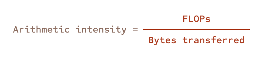
Arithmetic intensity tells us how much calculation we do for each byte moved; it does not directly tell us how fast an operation runs. When the processor spends much of its time waiting for data, memory bandwidth matters most. When it stays busy calculating, compute capacity matters more.

Grokking arithmetic intensity is key to understanding an LLM's different computational stages. Let's dive into some real examples.

Adding Two Matrices

Consider a simple matrix addition. To perform it on an accelerator, we need to read two matrices from memory, do the addition in the compute cores, and save the result back.

Let's do a real example.

Here, we load two numbers from memory (2 bytes each), execute a single FLOP to add them, then write the 2-byte result back to memory. This gives us 1 FLOP over 6 transferred bytes, for an arithmetic intensity of 0.167 FLOPs per byte.

Notice that as you increase the matrix size with the slider, both the calculation count and the bytes transferred grow in proportion. So in this example, although the total number of FLOPs increases for larger matrices, the relative arithmetic intensity stays the same.

Matrix Multiplication

Let's examine a different example. Matrix multiplication follows the same basic path: load two input matrices from memory, multiply and add their values in the compute units, then save the result matrix back to memory.

But unlike addition, each output value is built from an entire row of the first matrix and an entire column of the second. Hover over an output value to see the input values that contribute to it:

Notice what changes as you increase the matrix size. The accelerator still loads each input value once and writes each result once, but every loaded value can now contribute to more output values. The amount of data moved grows with the number of matrix entries, but the amount of arithmetic grows faster.

With matrix multiplications, we can increase arithmetic intensity even if only one of the input matrices changes. In the next example, we'll only make the second matrix interactive. Try the slider once more.

Even with one changing input, arithmetic intensity grows with input size! This relationship between input size and arithmetic intensity is key to understanding inference's different phases.

Arithmetic Intensity of Inference

Inference is a chain of many matrix multiplications. In this section, we'll apply the concepts we learned previously to understanding language models.

This article won't go into the full complexity of the language model architecture. But for our purposes, generating a token from a language model is basically a matrix operation between a model's weights and input tokens:

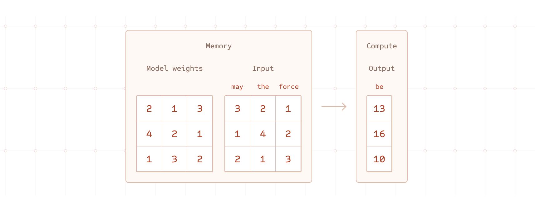
The left input matrix represents the model's weights. These are learned values that are fixed during inference. The right input matrix represents the input tokens that the model needs to process. We can think of each column as some numerical representation of a token.

To generate a single output token, the accelerator moves both the weights and inputs from memory into compute and performs a chain of matrix multiplications (simplified here as one operation). Press play to follow this process end-to-end below:

What looks like one continuous generation process is actually two distinct phases. First, the model processes the entire prompt (“may the force”) and produces the first response token, “be.” Then it generates the rest of the response one token at a time: “with” and “you.”

These phases are called prefill and decode, and they have very different arithmetic intensity profiles.

Note: 
Our examples follow one request. In production, servers often batch requests together, processing a new token for several users at once. This lets requests share the work of reading model weights. But larger batches can make each decode step take longer. Total throughput can rise while each user receives tokens more slowly.

Prefill

During prefill, the entire prompt is processed in parallel.

We learned earlier that larger matrix multiplications have higher arithmetic intensity because of more data reuse. We can make this more obvious with a longer input prompt:

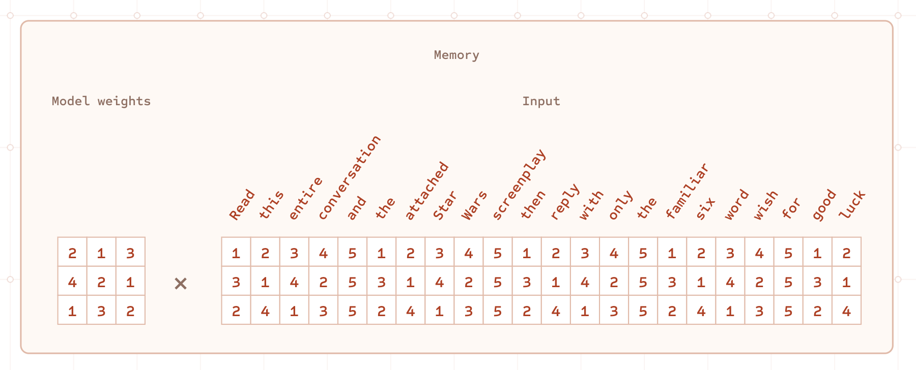
Real-world prompts can contain thousands or even hundreds of thousands of tokens. Uploading a 100-page PDF to a chatbot essentially generates a massive matrix calculation that needs to be processed.

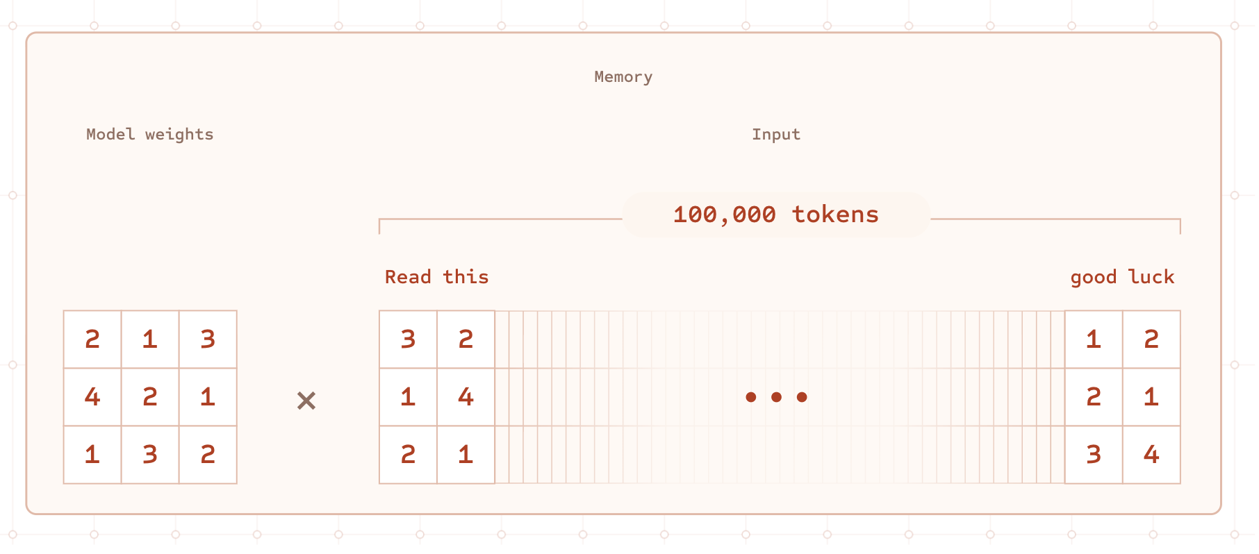
This is why prefill has relatively high arithmetic intensity! It's a large matrix operation.

Decode

During decode, tokens are generated one after another.

At first, it may seem like the model needs to run the entire growing sequence through the same large matrix multiplication every time. But language models avoid that with the KV cache.

The KV cache stores keys and values computed for earlier tokens, so we don’t have to calculate them again. As the context grows, reading and using the cache takes more work.

We won't go into the full complexity of the KV cache in this article, but you can treat the gray parts of the matrix as the cached data in each step of token generation. The result is a much smaller matrix operation.

Thanks to the cache, we avoid recomputing earlier tokens’ keys and values.

Note
The accelerator still reads cached keys and values from memory and uses them in attention. We show only the new token moving into compute to emphasize that earlier tokens’ keys and values are reused rather than recomputed. See the actual matrix operations in Hugging Face’s KV cache guide.

Prefill and Decode Have Different Profiles

In both phases, all of the model's weights must be brought to compute. That can mean moving hundreds of gigabytes or even terabytes of data. All of this has to be transferred to generate a single token, regardless of whether it's processing a million-token prompt during prefill or processing a single new input token during decode.

This is why prefill and decode have such different computational workloads despite having similar memory movement:

The Shared Scheduling Problem

So far, we've followed a single request through the system. In production, however, an inference server typically handles many requests concurrently. Some requests may be in the prefill stage, while others are already generating tokens in the decode stage.

When prefill and decode run on the same hardware, they can interfere with one another. Prefill is highly compute-intensive, which can stall ongoing decode requests.

A scheduler determines how requests are assigned and prioritized. Explore how different scheduling strategies affect request processing:

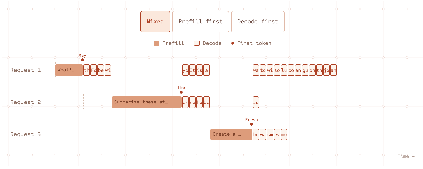
Prioritizing prefill helps new requests begin sooner, but can interrupt users whose responses are already streaming. Prioritizing decode helps existing responses stream smoothly, but can cause new prompts to wait for a long time before any response.

These decisions genuinely affect end-user experience. Switch between the three modes to see how each scheduling strategy affects a chatbot:

Aggregated systems—prefill and decode running on the same machines—must determine what outcome matters more to their application: getting new requests to their first token quickly, keeping active responses streaming smoothly, or maximizing overall throughput.

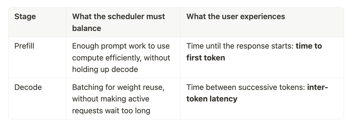
Disaggregation

Let's recap what we've learned so far:

Accelerators (hardware) perform arithmetic. This happens by bringing data from memory to compute and writing data back.
For the same amount of data moved, some workloads perform more arithmetic than others.
Prefill and decode are different phases of inference.
Prefill is computationally involved due to processing multiple tokens in parallel.
Decode processes one new token per request at each step, but still needs substantial memory access for model weights and the KV cache.
Balancing these two workloads on the same hardware is difficult and requires trade-offs at scale.

Disaggregation is a systems design pattern. It identifies work with different resource needs, then operates those workloads separately rather than forcing them to share a single pool of hardware.

A disaggregated system uses two separate hardware pools: one for prefill and one for decode. Select “Disaggregated” to see how this changes the schedule.

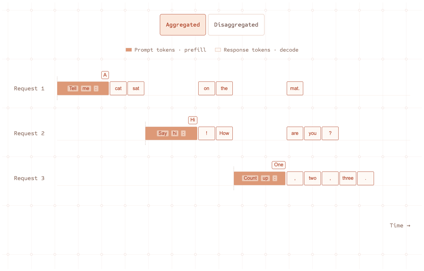
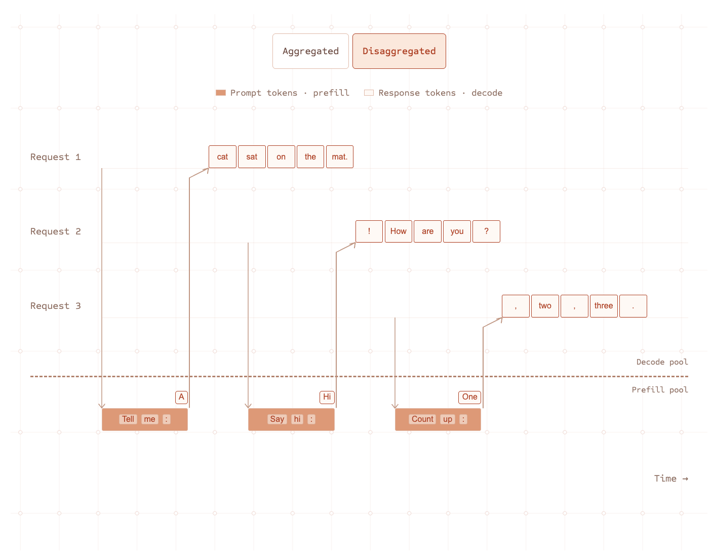
In a shared pool, time to first token and inter-token latency are directly coupled. Starting a new prompt can delay active responses; protecting active responses can leave new prompts waiting.

Disaggregation is a lot more than "smoother streaming". More fundamentally, disaggregation changes the control interface for the serving system.

More Control Over Trade-offs

In a shared pool, capacity, batching, and scheduling decisions affect prefill and decode together. Once the stages are separated, operators can tune each one independently—allocating hardware, setting batching policies, and prioritizing latency or throughput according to the product’s requirements.

For example, a system with strict time-to-first-token targets can reserve more capacity for prefill, so incoming prompts start promptly without consuming decode capacity. A system that prioritizes a smooth streaming experience can give decode a larger or more tightly scheduled pool, keeping active responses moving even when prompt traffic spikes.

The point is that these pools can be scaled individually. Click different scenarios to see how pools might be scaled to meet different demands:

You can see how disaggregation allows the system to adapt to different workload shapes.

But separating the stages introduces a new need: data transfer between the pools. The most important new piece of that design is the transfer of the KV cache.

The KV Transfer

After prefill builds the KV cache, the system transfers that state to the decode pool, where it is loaded into memory before generation can continue.

Unlike the model weights, which are already loaded in both pools, the KV cache is request-specific data. Handoff adds some network and coordination overhead, which is why disaggregation is most compelling at scale: with enough concurrent work, the gains from independently sizing and scheduling prefill and decode can outweigh the cost of transferring state and operating separate pools.

Once prefill has processed a prompt, decode needs the request-specific state that prefill created. Both pools already have the model weights, so the state that must cross the boundary is the KV cache.

Follow one request below to see that handoff:

Separating the phases adds costs too. The KV cache must travel between pools, and either pool can sit idle if their capacities do not match demand. Latency also depends on whether the cache is sent across colocated machines or across regions. Ultimately the operator must decide whether the latency addition is acceptable.

Heterogeneous Disaggregation

So far, our examples have shown separation of prefill and decode into two pools of the same hardware.

Disaggregation is even more powerful when introducing heterogeneous hardware combinations. The question is no longer simply which accelerator should run the model, but which combination of accelerators best serves this workload.

If each pool can be assigned to different hardware, it makes specialized hardware compelling: an accelerator that is exceptional at one dimension—such as prompt processing, memory bandwidth, token speed, or cost efficiency—can boost performance beyond disaggregating with a single type of chip.

Cerebras has exceptionally high aggregate on-chip memory bandwidth. Its wafer-scale architecture is designed around fast access to local memory, making it particularly well suited to the token-by-token portion of inference.

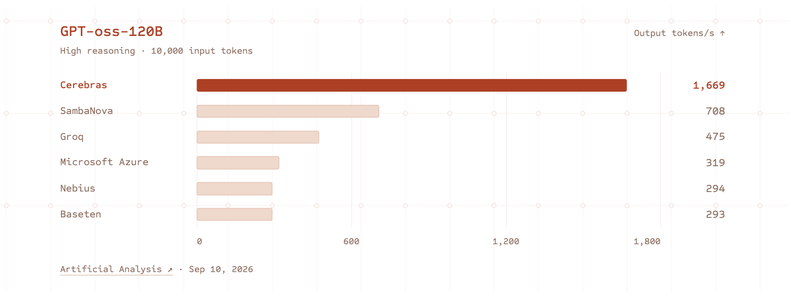
Why are some accelerators better at decode?

Remember what makes decode different: we move a lot of data to produce just one new token. Its arithmetic intensity is relatively low, so adding more raw FLOP capacity doesn’t necessarily make tokens arrive faster. The compute needs to be fed with more data from memory.

On a GPU, model data resides primarily in high-bandwidth memory (HBM). Before compute units can use it, data is staged through smaller, faster on-chip memories and caches, including SRAM. This memory hierarchy provides large capacity alongside fast local storage, but data still has to travel from shared external memory toward the compute cores.

Cerebras takes a different approach: it distributes SRAM alongside compute across the entire wafer. That gives compute fast access to nearby memory:

This wafer-scale design gives Cerebras exceptionally high aggregate memory bandwidth:

Goals of Disaggregation

Homogeneous and heterogeneous disaggregation provide different benefits.

While homogeneous systems commonly aim to improve responses by smoothing token generation, heterogeneous systems are optimized to get the most value out of the specialized hardware. In Cerebras' case, it provides extreme speed without sacrificing throughput.

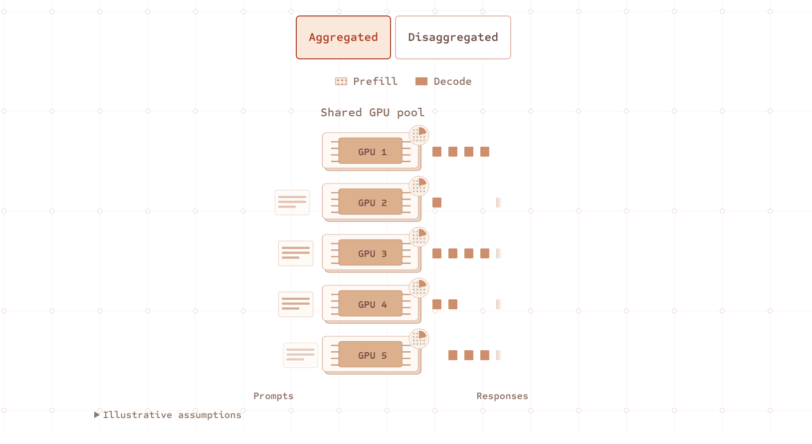
Consider an aggregated system with five GPUs, each spending 80% of its execution time on prefill and 20% on decode. An active response advances only when its GPU performs a decode step. Spending four-fifths of the time on prefill slows the average pace of output token generation.

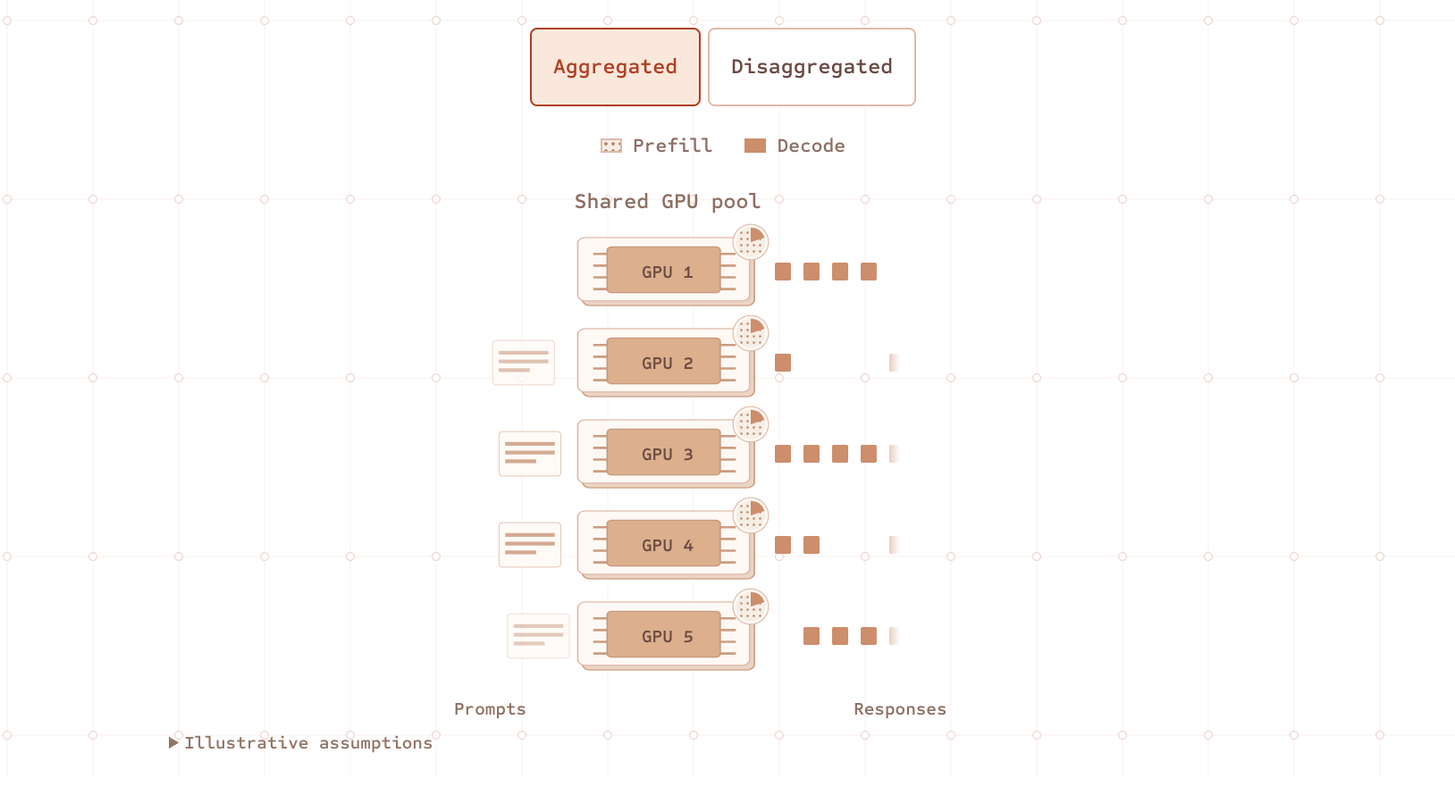
Across the five GPUs, decode accounts for one GPU’s worth of execution time. In this idealized steady state, disaggregation assigns that work to one dedicated GPU and prefill to the other four. The decode GPU can advance responses without competing with prefill, improving token cadence with the same GPU count.

The more time shared GPUs spend on prefill, the larger the improvement. If GPUs already spend most of their time on decode, there's less interference to remove in a homogeneous system. But reducing interference is only one reason to disaggregate. In a heterogeneous system, disaggregation optimizes for better hardware specialization.

Suppose five Cerebras WSEs currently handle both phases. By moving prefill to a separate accelerator pool, it allows the wafers to specialize in decode, where their capacity is most valuable.

This is a gain in throughput per WSE, enabled by additional prefill hardware.

Agentic applications are a compelling fit for heterogeneous disaggregation. They often involve long, multi-turn workflows, with context growing across model calls. As agents take on longer and more consequential tasks, delays at each step compound. Fast inference becomes essential to how responsive an agent feels and how quickly tasks are completed.

Cerebras Disaggregation unlocks the ability to scale inference without compromising world-class interactivity.

Cerebras Uses Disaggregation to Scale Ultrafast Tokens

Demand for ultrafast generation is growing quickly. As more applications become agentic, the limiting resource is increasingly not just total model capacity, but the number of fast tokens we can deliver to users at once.

At Cerebras, we are building heterogeneous inference systems to meet that demand. The goal is not simply to increase aggregate throughput—it is to scale the volume of inference while preserving the ultrafast token speeds that make applications feel instant.

In a traditional aggregated system, increasing capacity meant deploying more hardware. By leveraging partner accelerators to handle prompt processing, we've increased capacity by 5× in early tests with the same WSE footprint.

We have announced partnerships with multiple hardware partners to bring more ultrafast tokens to the market, reflecting our belief that heterogeneous hardware will be a core inference strategy going forward.

What's Next

In the next posts, we’ll dive deeper into bringing heterogeneous disaggregation to production. We’ll explore the hardware and software stacks involved, and the economic trade-offs of deploying disaggregated inference at scale.

Follow us on X to be notified when the next post goes live!

Disaggregated Inference from the Ground up